Purpose of This Page
This page walks through the minimal workflow needed to start using BayesRTMB.
It covers the following topics.
- Write a small model with
rtmb_code() - Create a model object with
rtmb_model() - Estimate the model with
optimize()andsample() - Visualize the posterior distribution from MCMC
- Use wrapper functions for multiple regression and interactions
- Run a frequentist t test with
classic() - Compute a Bayes factor using a JZS prior and MCMC
Detailed model writing, mixed models, GLMMs, model comparison, and function-level reference material are covered in other vignettes, especially the Analysis Reference.
0. Installation and Environment Check
BayesRTMB can be installed from CRAN.
install.packages("BayesRTMB")The development version can be installed from GitHub. If you use
pak, install it as follows.
install.packages("pak")
pak::pak("norimune/BayesRTMB")
If you use remotes, install it as follows.
install.packages("remotes")
remotes::install_github("norimune/BayesRTMB")
Windows Users
BayesRTMB uses RTMB / TMB internally. For ordinary use, Windows users can install the CRAN binary package without Rtools. Rtools is only needed for source installation, development, or compiling custom TMB C++ templates.
If you install BayesRTMB from source, you can check whether Rtools is available with the following code.
pkgbuild::check_build_tools(debug = TRUE)If this returns TRUE, or reports that build tools are
available, your source-install setup is ready. If Rtools is not found,
install the Rtools version that matches your R version, then restart R
or RStudio.
1. Write a Minimal Model
We start with a small binomial model. Suppose that 6 successes were observed out of 10 trials.
library(BayesRTMB)

Trial <- 10
Y <- 6

dat <- list(Trial = Trial, Y = Y)

code <- rtmb_code(
  parameters = {
    theta <- Dim(lower = 0, upper = 1)
  },
  model = {
    Y ~ binomial(Trial, theta)
    theta ~ beta(1, 1)
  }
)
The parameters block declares the parameters to
estimate. Here, theta is defined as a parameter constrained
between 0 and 1.
The model block specifies the sampling distribution and
prior distribution. Y ~ binomial(Trial, theta) says that
the number of successes Y follows a binomial
distribution.
2. Create a Model Object
Pass the data and model code to rtmb_model() to create a
model object for estimation.
mdl <- rtmb_model(dat, code)## Pre-checking model code...
## Checking RTMB setup...At this stage, estimation has not yet been run. mdl is
an RTMB_Model object that stores the model definition and
data.
3. Run MAP Estimation
Use optimize() when you want a fast point estimate. In
BayesRTMB, this is treated as MAP estimation when priors are present,
and as something close to maximum likelihood estimation when flat priors
are used.
fit_map <- mdl$optimize()
fit_map
## Starting RTMB optimization...
##
## Call:
## MAP Estimation via RTMB
##
## Negative Log-Posterior: 1.38
## Approx. Log Marginal Likelihood (Laplace): -2.33
##
## Point Estimates and 95% Wald CI:
## variable Estimate Std. Error Lower 95% Upper 95%
## theta 0.60000 0.15492 0.29740 0.84166 In this example, the estimated success probability theta
is 0.60.
4. Inspect the Posterior with MCMC
Use sample() when you want to inspect the full posterior
distribution. The settings below are intentionally short for a quick
start. For real analyses, use more iterations.
set.seed(1)

fit_mcmc <- mdl$sample(
  sampling = 200,
  warmup = 200,
  chains = 2
)

fit_mcmc$summary()
## Starting sequential sampling (chains = 2)...
## chain 1 started...
## chain 1: iter 100 warmup
## chain 1: iter 200 warmup
## chain 1: iter 300 sampling
## chain 1: iter 400 sampling
## chain 2 started...
## chain 2: iter 100 warmup
## chain 2: iter 200 warmup
## chain 2: iter 300 sampling
## chain 2: iter 400 sampling
## variable mean sd map q2.5 q97.5 ess_bulk ess_tail rhat
## lp -3.30 0.69 -2.88 -5.25 -2.80 132 188 1.00
## theta 0.58 0.13 0.60 0.32 0.83 165 177 1.01 The MCMC summary reports the mean, standard deviation, posterior quantiles, ESS, and R-hat. As a rough diagnostic, R-hat should be close to 1 and ESS should be sufficiently large.
Parallel MCMC
Ordinary MCMC can be run without additional setup. However, if you
use parallel MCMC with sample(parallel = TRUE), the
suggested package future is required.
install.packages("future")
fit_mcmc <- mdl$sample(
  sampling = 1000,
  warmup = 1000,
  chains = 4,
  parallel = TRUE
)
5. Visualize MCMC Results
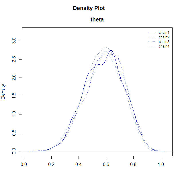
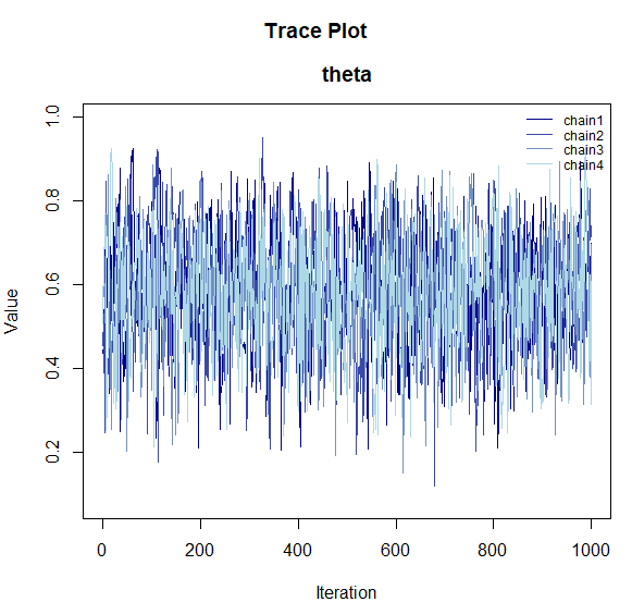
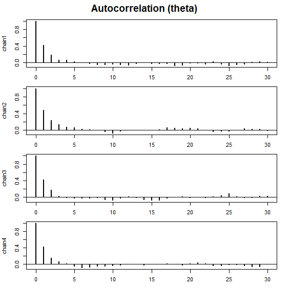
MCMC results should be checked visually as well as numerically. Use
draws() to extract samples for a target parameter, then
inspect densities, traces, autocorrelation, and intervals.
theta_draws <- fit_mcmc$draws("theta")

plot_dens(theta_draws)
plot_trace(theta_draws)
plot_acf(theta_draws)
Each plot has a different role.
-
plot_dens()shows the shape of the posterior distribution. -
plot_trace()checks whether the chains mix well. -
plot_acf()checks whether autocorrelation is too strong.
For example, these functions produce plots like the following.
6. Multiple Regression with a Wrapper Function
For standard analyses, you can start from a wrapper function instead
of writing rtmb_code() yourself.
Here we use the debate data and fit a multiple
regression model in which satisfaction sat is explained by
talk, perf, and their interaction.
data(debate)

mdl_lm <- rtmb_lm(
  sat ~ talk * perf,
  data = debate,
  gmc = "all",
  prior = prior_normal()
)

fit_lm <- mdl_lm$optimize(
  se_method = "sampling",
  num_samples = 1000,
  seed = 1
)
fit_lm
## Starting RTMB optimization...
##
## Using simulation-based error propagation (1000 samples)...
##
##
## Call:
## MAP Estimation via RTMB
##
## Negative Log-Posterior: 402.24
## Approx. Log Marginal Likelihood (Laplace): -414.02
##
## Point Estimates and 95% Sampling-based CI:
## variable Estimate Std. Error Lower 95% Upper 95%
## Intercept_c 3.43325 0.05232 3.33253 3.53604
## b[talk] 0.26572 0.05305 0.15585 0.36839
## b[perf] 0.14054 0.02924 0.08274 0.19857
## b[talk:perf] 0.13022 0.03063 0.06780 0.19111
## sigma 0.87135 0.03629 0.80181 0.94375
## Intercept 3.41638 0.05254 3.31562 3.51660 Use plot_forest() when you want to view the coefficients
at a glance.
fit_lm$draws(c("b[talk]", "b[perf]", "b[talk:perf]")) |>
  plot_forest(point_estimate = "MAP")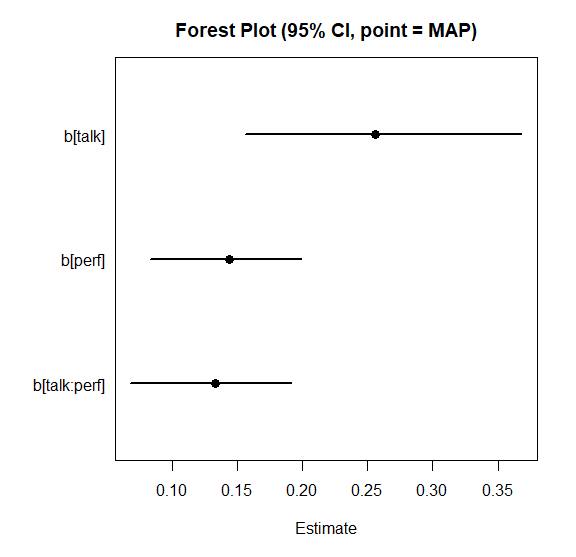
7. Plot an Interaction
Interactions are often difficult to interpret from a coefficient
table alone. Use conditional_effects() to visualize
predicted values.
ce <- conditional_effects(fit_lm, effect = "talk:perf")
plot(ce)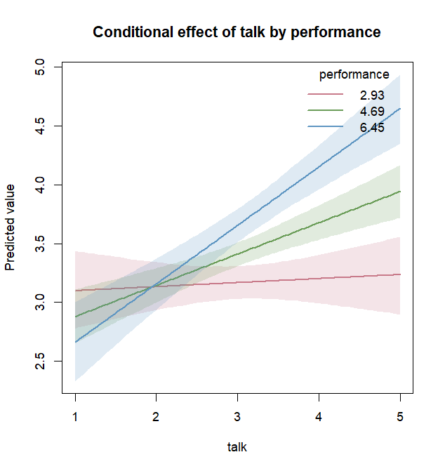
With effect = "talk:perf", you can see how the effect of
talk changes depending on the value of
perf.
For a more detailed look, use simple_effects() to
calculate simple slopes.
simple_effects(fit_lm, effect = "talk:perf")8. Run a Frequentist t Test
BayesRTMB wrapper functions can also be used for frequentist
analyses. Calling classic() on a t test with
prior_flat() displays results in a form close to an
ordinary t test.
mdl_t <- rtmb_ttest(
  sat ~ cond,
  data = debate,
  prior = prior_flat()
)

fit_t_classic <- mdl_t$classic()
fit_t_classic
## Pre-checking model code...
## Checking RTMB setup...
## Starting RTMB optimization...
##
## Call:
## Classical estimation via ttest
##
## Log-Likelihood: -421.320, AIC: 848.640, BIC: 842.640
##
## Point Estimates and Confidence Intervals:
## Estimate Std. Error Lower 95% Upper 95% df t value Pr
## diff -0.37333 0.11297 -0.59564 -0.15102 298 -3.30484 .00107 **
## delta -0.38161 0.11652 -0.61092 -0.15230 298 NA
## total_mean 3.43333 0.05648 3.32218 3.54449 298 NA
## sd 0.97831 0.04007 0.90254 1.06044 298 NA
## mean0 3.24667 0.07988 3.08947 3.40386 298 NA
## mean1 3.62000 0.07988 3.46280 3.77720 298 NAHere, diff is the difference between the two group
means, and delta is the standardized effect size. Use
classic() when you want to inspect a BayesRTMB model as a
frequentist analysis.
9. Compute a Bayes Factor with a JZS Prior
The same t test can also be used to compute a Bayes factor by placing
a Cauchy prior on the effect size delta through the JZS
prior. BayesRTMB also applies the Jeffreys scale prior
to the residual standard deviation; for an unequal-variance test, it is
applied separately to both group standard deviations.
mdl_t_jzs <- rtmb_ttest(
  sat ~ cond,
  data = debate,
  prior = prior_jzs()
)

set.seed(2)

fit_t_jzs <- mdl_t_jzs$sample()

bf <- fit_t_jzs$bayes_factor(fixed = list(delta = 0))
bf
## --- Bayes Factor Analysis (Bridge Sampling) ---
## Bayes Factor (BF12) : 21.4323
## Log Bayes Factor : 3.0649 (Approx. Error = 0.0022)
## Evidence : Strong evidence for Model 1
## Comparison model : Parameters fixed at list(delta = 0) fixed = list(delta = 0) specifies a comparison against
the null model where the effect size is fixed at 0. In this example,
Model 1, the model that estimates the effect size, is
supported.
For real analyses, use more MCMC samples than shown here and check that the Bayes factor is stable.
Next Steps
This page covered only the entry points to BayesRTMB. Continue with the page that matches your purpose.
Wrapper Functions
Learn how to run standard analyses such as regression, GLM, mixed models, t tests, correlations, factor analysis, and IRT with wrapper functions.Hierarchical Models and GLMMs
Learn how to usertmb_glmer()for hierarchical models, GLMMs, residual correlation, conditional effects, priors, and ANOVA-style workflows.Writing Model Codes
Learn how to write custom models with thesetup,parameters,transform,model, andgenerateblocks.RTMB Internals and Inference Algorithms
Learn about internal processing such as MAP estimation, Laplace approximation, MCMC, and variational inference.Analysis Reference
Check fit-object methods, model-comparison tools, fixed parameters, distributions, and AD-taping notes.