In BayesRTMB, you can freely define models using the
rtmb_code block, but we also provide wrapper
functions to quickly execute common statistical analyses (like
t-tests, regressions, and factor analysis).
These functions allow you to specify models with syntax similar to
standard R functions such as lm() and mixed-model formula
interfaces, while fully utilizing the powerful estimation features of
BayesRTMB (MCMC, MAP, ADVI).
This page introduces the usage of the main wrapper functions.
1. rtmb_ttest (Bayesian t-test)
This function is for examining the difference in means between two
groups. rtmb_ttest is designed to easily perform
effect size (delta) estimation and Bayes factor
calculation, in addition to standard t-tests.
First, let’s generate some sample data and analyze it.
library(BayesRTMB)
set.seed(123)

# Data generation (2 groups)
y1 <- rnorm(30, mean = 0, sd = 1)
y2 <- rnorm(30, mean = 1, sd = 1)

# Method passing vectors directly
mdl_ttest <- rtmb_ttest(y1, y2, prior = prior_jzs())

# Method using formula format (when you have a dataframe)
# df <- data.frame(Y = c(y1, y2), group = rep(c("A", "B"), each = 30))
# mdl_ttest <- rtmb_ttest(Y ~ group, data = df, prior = prior_jzs())

# MCMC estimation
fit_ttest <- mdl_ttest$sample()
fit_ttest$summary()
## variable mean sd map q2.5 q97.5 ess_bulk ess_tail rhat
## lp -88.05 1.23 -87.08 -91.16 -86.63 1543 2467 1.00
## delta 1.24 0.30 1.25 0.65 1.84 1830 1654 1.01
## mean 0.57 0.12 0.58 0.34 0.81 3058 2436 1.00
## sd 0.93 0.09 0.92 0.78 1.13 2371 2755 1.00
## diff 1.15 0.25 1.11 0.64 1.63 2309 1695 1.01
## mean0 -0.00 0.17 -0.01 -0.34 0.34 2645 2468 1.00
## mean1 1.14 0.17 1.14 0.80 1.49 2507 2364 1.00 Checking the Generated Code
You can check what rtmb_code the wrapper function
generated internally by using the print_code() method on
the model object. This can be used as a reference if you want to extend
the wrapper’s model into your own custom model.
# Display the internally generated RTMB code
mdl_ttest$print_code()
## === RTMB Model Code ===
##
## rtmb_code(
## parameters = {
## total_mean = Dim(1)
## sd = Dim(1, lower = 0)
## delta = Dim(1)
## },
## transform = {
## diff <- delta * sd
## mean0 <- total_mean + diff/2
## mean1 <- total_mean - diff/2
## },
## model = {
## Y1 ~ normal(mean0, sd)
## Y2 ~ normal(mean1, sd)
## delta ~ cauchy(0, r)
## lp <- lp - log(sd)
## }
## )The lp <- lp - log(sd) term applies the Jeffreys
scale prior
used by the JZS t-test.
Calculating the Bayes Factor
By using the bayes_factor() method, you can compute a
comparison (Bayes factor) against a null model where the effect size is
.
# Compare with the model where effect size delta = 0
bf <- fit_ttest$bayes_factor(fixed = list(delta = 0))
bf
## Bayes Factor (BF12) : 4777.563
## Log Bayes Factor : 8.4717 (Approx. Error = 0.0039)
## Interpretation : Decisive evidence for Model 1 2. rtmb_lm (Linear Regression Analysis)
You can perform linear regression with a format identical to standard
lm(). Here, we use the debate data included in
the package (simulated data regarding debate sat).
data(debate)

# Model predicting sat using talk and skill
mdl_lm <- rtmb_lm(sat ~ talk + skill, data = debate)

# Quick check via MAP estimation
fit_lm <- mdl_lm$optimize()
fit_lm$summary()
## Call:
## MAP Estimation via RTMB
##
## Negative Log-Posterior: 416.94
## Approx. Log Marginal Likelihood (Laplace): -425.12
##
## Point Estimates and 95% Wald CI:
## variable Estimate Std. Error Lower 95% Upper 95%
## Intercept 2.14693 0.20761 1.74001 2.55384
## b[talk] 0.28612 0.05434 0.17961 0.39264
## b[skill] 0.20106 0.06604 0.07162 0.33050
## sigma 0.92284 0.03725 0.85265 0.99880
## Intercept_c 3.43324 0.05333 3.32871 3.53777 Recommended Settings for Weakly Informative Priors
When calculating Bayes factors (using Bridge Sampling or
the bayes_factor method), the choice of priors strongly
influences the results. BayesRTMB recommends automatically configuring
appropriate Weakly Informative Priors by setting
use_weak_info = TRUE and specifying the theoretical minimum
and maximum values of the objective variable in
y_range.
# Create a model using weakly informative priors (assuming sat ranges from 1 to 5)
mdl_lm_weak <- rtmb_lm(sat ~ talk + skill,
  data = debate,
  use_weak_info = TRUE,
  y_range = c(1, 5)
)
mdl_lm_weak$print_code()
## === RTMB Model Code ===
##
## rtmb_code(
## setup = {
## N <- length(Y)
## K <- ncol(X)
## half_d_y <- diff(y_range)/2
## base_scale <- half_d_y * weak_info_prior$sd_ratio
## alpha_prior_sd <- half_d_y
## mid_y <- mean(y_range)
## sigma_rate <- 1/base_scale
## tau_rate <- 1/base_scale
## X_mean <- apply(X, 2, mean)
## X_sd <- apply(X, 2, sd)
## beta_prior_sd <- weak_info_prior$max_beta * base_scale/X_sd
## X_c <- X - rep(1, N) %*% t(X_mean)
## },
## parameters = {
## Intercept_c <- Dim(1)
## b <- Dim(K)
## sigma <- Dim(1, lower = 0)
## },
## transform = {
## Intercept <- Intercept_c - sum(X_mean * b)
## },
## model = {
## # Transform
## eta <- as.vector(Intercept_c + X_c %*% b)
## # Likelihood (Data)
## Y ~ normal(eta, sigma)
## # Priors
## sigma ~ exponential(sigma_rate)
## Intercept_c ~ normal(mid_y, alpha_prior_sd)
## b ~ normal(0, beta_prior_sd)
## }
## )3. rtmb_glm (Generalized Linear Models)
By specifying the family argument, you can perform
logistic regression, Poisson regression, etc. As an example, we will
execute a logistic regression predicting the experimental cond (cond: 0
or 1).
# Logistic regression (family = "bernoulli")
mdl_glm <- rtmb_glm(cond ~ sat + skill,
  data = debate,
  family = "bernoulli"
)

fit_glm <- mdl_glm$sample()
fit_glm$summary()
variable mean sd map q2.5 q97.5 ess_bulk ess_tail rhat
## lp -213.72 1.24 -212.80 -216.90 -212.31 1567 2449 1.00
## Intercept -1.35 0.50 -1.32 -2.31 -0.38 3740 2794 1.00
## b[sat] 0.40 0.13 0.38 0.16 0.64 3127 2838 1.00
## b[skill] -0.01 0.15 0.01 -0.30 0.28 3445 2925 1.00
## Intercept_c -0.00 0.12 -0.03 -0.23 0.23 4129 2544 1.00 Available Distributions (family)
In rtmb_glm and rtmb_glmer, the following
distributions can be specified. Standard link functions are configured
internally for each distribution.
family |
Link Function | Description |
|---|---|---|
gaussian |
identity | Normal distribution. For standard regression analysis. |
lognormal |
log | Log-normal distribution. For data that takes positive values. |
student_t |
identity | t-distribution. Useful when you want to suppress the impact of outliers. |
gamma |
log | Gamma distribution. For positive, skewed data. |
bernoulli |
logit | Bernoulli distribution. For binary 0/1 data. |
binomial |
logit | Binomial distribution. For data representing counts of success/trials. |
poisson |
log | Poisson distribution. For count data. |
neg_binomial |
log | Negative binomial distribution. For overdispersed count data. |
ordered |
logit | Ordered logistic regression. For ordinal categorical data. |
4. rtmb_glmer (Generalized Linear Mixed Models)
You can handle models including random effects (varying effects)
using the (1 | group) notation, similar to the
lme4 package. Let’s build a model taking into account that
individual sat varies depending on the group they belong to.
# Random intercept model
mdl_glmer <- rtmb_glmer(sat ~ talk + (1 | group),
  data = debate
)

# When including random effects, optimize() with Laplace approximation is fast
opt_glmer <- mdl_glmer$optimize(laplace = TRUE)
opt_glmer$summary()
## Call:
## MAP Estimation via RTMB
##
## Negative Log-Posterior: 404.65
## Approx. Log Marginal Likelihood (Laplace): -412.59
## Note: Random effects are stored in $random_effects
##
## Point Estimates and 95% Wald CI:
## variable Estimate Std. Error Lower 95% Upper 95%
## Intercept 2.60450 0.17902 2.25363 2.95537
## b[talk] 0.27441 0.05477 0.16706 0.38176
## sigma 0.77389 0.03867 0.70170 0.85351
## sd[Int] 0.51833 0.06587 0.40406 0.66492
## Intercept_c 3.43322 0.06846 3.29904 3.56740 Regularization
In rtmb_lm, rtmb_glm, and
rtmb_glmer, you can use regularization. Regularization is a
method that shrinks the coefficients of excessive parameters towards 0,
allowing for the construction of more parsimonious models with high
predictive power.
In the BayesRTMB package, you can select the horseshoe
prior (rhs) or the spike-and-slab prior (ssp)
using the penalty option. rhs is relatively
easier to estimate, but coefficients with small effects do not shrink
exactly to 0. ssp is somewhat heavier to estimate, but it
can shrink coefficients completely to 0.
When using regularization, you must also use weakly informative
priors, which means you need to input the range of the objective
variable. Since our data uses a 5-point scale, we input
c(1, 5). MAP estimation often struggles with regularized
models, so it’s better to use MCMC.
mdl_glmer <-
  rtmb_glmer(
    sat ~ talk + perf + skill + cond + (1 | group),
    data = debate,
    penalty = "ssp",
    y_range = c(1, 5)
  )

mcmc_glmer <- mdl_glmer$sample(parallel = TRUE)
mcmc_glmer
mcmc_glmer$draws("b[cond]") |> plot_dens()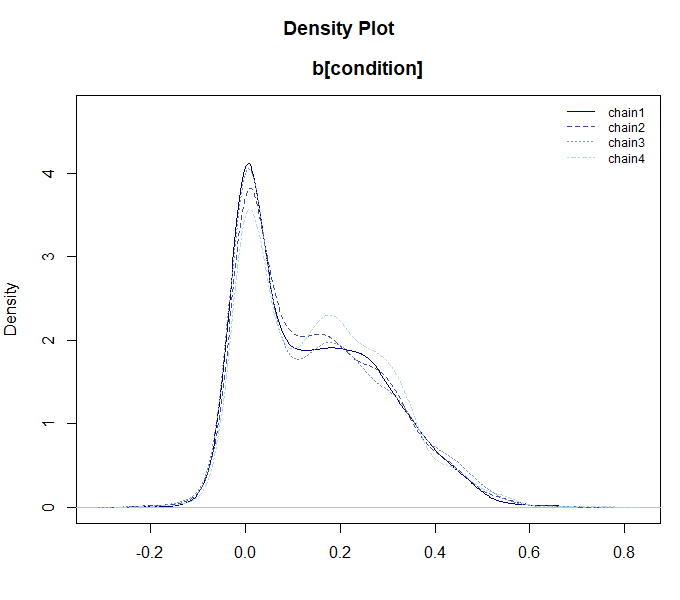
5. Post-Estimation Analysis (Interaction & Visualization)
After fitting a regression model (LM, GLM, GLMER), you can use
conditional_effects() and simple_effects() to
analyze and visualize the results. These methods are available for MCMC
fits and can also be used with MAP or classic fits when the fitted
object contains the standard errors or sampling-based uncertainty needed
for the requested summary.
Visualization with conditional_effects()
The conditional_effects() function is used to visualize
the predicted values of a model. It is particularly powerful for
understanding interaction effects.
# Linear regression with interaction between talk and cond
mdl_int <- rtmb_lm(sat ~ talk * perf, data = debate)
fit_int <- mdl_int$sample()

# Visualize the interaction effect
# For continuous moderators, it automatically shows Mean +/- 1SD
ce <- conditional_effects(fit_int, effect = "talk:perf")
plot(ce)
Simple Effects Analysis with simple_effects()
While conditional_effects() provides a visual overview,
simple_effects() allows you to statistically examine the
effect of a focal variable at specific levels of a moderator.
- Simple Slopes: When the focal variable is continuous.
- Pairwise Contrasts: When the focal variable is categorical.
# Calculate simple slopes of 'talk' for each level of 'cond'
se <- simple_effects(fit_int, effect = "talk:perf")
print(se)
## --- Simple Effects Analysis ---
## moderator perf term estimate lower upper
## perf 2.930 Slope of talk 0.038 -0.118 0.191
## perf 4.690 Slope of talk 0.266 0.161 0.369
## perf 6.450 Slope of talk 0.494 0.354 0.631By default, for continuous moderators, it evaluates the effect at the
Mean and Mean +/- 1SD. You can change this behavior by specifying the
sd_multiplier argument.
6. rtmb_corr (Correlation Matrix Estimation)
This function is for estimating the correlation relationships between variables. Here, we will introduce both a 2-variable case and a full correlation matrix case using a portion of the Big Five personality data.
2-Variable Correlation and Bayes Factor
We estimate the correlation between two variables (e.g., extraversion items BF1 and BF6), and calculate a Bayes factor testing the null hypothesis of zero correlation ().
data(BigFive)

# Correlation between BF1 and BF6
mdl_corr2 <- rtmb_corr(BigFive[, c("BF1", "BF6")])
mcmc_corr2 <- mdl_corr2$sample()
mcmc_corr2$summary()
## variable mean sd map q2.5 q97.5 ess_bulk ess_tail rhat
## lp -493.27 1.55 -492.22 -497.08 -491.16 1799 2658 1.00
## corr[rho] -0.60 0.05 -0.60 -0.69 -0.50 2365 2539 1.00
## mean[BF1] 3.56 0.08 3.56 3.39 3.72 3031 2914 1.00
## mean[BF6] 2.71 0.09 2.73 2.54 2.89 2978 2872 1.00
## sd[BF1] 1.10 0.06 1.07 0.99 1.22 3151 3313 1.00
## sd[BF6] 1.15 0.06 1.16 1.04 1.28 3072 2477 1.00
# Compare against the zero-correlation model (fixed = list(corr = 0))
bf_corr <- mcmc_corr2$bayes_factor(fixed = list(corr = 0))
bf_corr
Bayes Factor (BF12) : 6.839475e+15
Log Bayes Factor : 36.4615 (Approx. Error = 0.0043)
Interpretation : Decisive evidence for Model 1 Correlation Matrix Estimation
If you specify multiple variables at once, the entire correlation matrix is estimated.
# Estimate the correlation matrix of 5 variables
mdl_corr_mat <- rtmb_corr(BigFive[, 1:5])
opt_corr_mat <- mdl_corr_mat$optimize()
opt_corr_mat$summary()
## Call:
## MAP Estimation via RTMB
##
## Negative Log-Posterior: 1254.77
## Approx. Log Marginal Likelihood (Laplace): -1289.58
##
## Point Estimates and 95% Wald CI:
## variable Estimate Std. Error Lower 95% Upper 95%
## corr[BF1,BF1] 1.00000 0.00000 1.00000 1.00000
## corr[BF2,BF1] 0.09243 0.07555 -0.05565 0.24050
## corr[BF3,BF1] 0.09382 0.07552 -0.05420 0.24184
## corr[BF4,BF1] 0.08807 0.07562 -0.06014 0.23629
## corr[BF5,BF1] -0.02158 0.07619 -0.17090 0.12775
## corr[BF1,BF2] 0.09243 0.07555 -0.05565 0.24050
## corr[BF2,BF2] 1.00000 0.00000 1.00000 1.00000
## corr[BF3,BF2] -0.03374 0.07610 -0.18289 0.11542
## corr[BF4,BF2] -0.13588 0.07481 -0.28250 0.01074
## corr[BF5,BF2] -0.08526 0.07567 -0.23357 0.06306 7. rtmb_fa (Exploratory Factor Analysis)
Estimates the common latent factors behind observed variables.
Factor Rotation
Factor analysis can be slightly time-consuming with MCMC, making MAP
estimation faster and easier to use. Factor rotation can be performed
via the rotate option. The rotated factor loadings will
have the rotation name appended, like _promax. Because the
rotated factor loadings are placed in the generate block,
MAP does not calculate standard errors for them by default. By
specifying se_sampling = TRUE, you can compute their
standard errors as well.
# 3-factor model, specifying Promax rotation
mdl_fa <- rtmb_fa(BigFive, nfactors = 5, rotate = "promax")

opt_fa <- mdl_fa$optimize(se_sampling = TRUE)

# Check the factor loadings (L), etc.
opt_fa$summary()
## Call:
## MAP Estimation via RTMB
##
## Negative Log-Posterior: 4791.18
## Approx. Log Marginal Likelihood (Laplace): -5016.21
##
## Point Estimates and 95% Wald CI:
## variable Estimate Std. Error Lower 95% Upper 95%
## L_promax[BF1,1] 0.86657 0.05905 0.72847 0.95902
## L_promax[BF2,1] 0.02202 0.05325 -0.07631 0.12786
## L_promax[BF3,1] -0.09276 0.06886 -0.20404 0.06562
## L_promax[BF4,1] 0.04927 0.06391 -0.07333 0.17433
## L_promax[BF5,1] -0.02101 0.04856 -0.11742 0.07748
## L_promax[BF6,1] -0.80459 0.05957 -0.89651 -0.66314
## L_promax[BF7,1] -0.01111 0.05307 -0.11843 0.08566
## L_promax[BF8,1] -0.07429 0.05917 -0.16758 0.06246
## L_promax[BF9,1] -0.08225 0.07363 -0.23533 0.05242
## L_promax[BF10,1] 0.03086 0.05210 -0.07256 0.13540 The sort_loadings() function is useful to sort and
display the rotated factor loadings nicely.
opt_fa$generate$L_promax |> sort_loadings()## V1 V2 V3 V4 V5
## V1 .867 -.117 -.179 .089 .057
## V6 -.805 .000 .048 .200 -.065
## V11 .584 .087 .126 .169 -.197
## V16 .516 .087 .276 -.009 .040
## V2 .022 -.806 -.076 -.013 .043
## V7 -.011 -.800 -.175 -.054 .002
## V12 .065 -.797 -.045 -.083 -.088
## V17 .007 -.763 .070 .009 -.012
## V8 -.074 .172 .830 -.044 -.061
## V3 -.093 .044 .533 .101 .060
## V18 -.036 -.196 .512 -.156 -.066
## V13 -.005 -.078 .488 -.121 .154
## V4 .049 .118 -.080 .607 .058
## V14 -.096 -.037 -.031 .586 -.022
## V19 .094 .054 .001 .506 -.085
## V9 -.082 .064 -.059 .463 .019
## V5 -.021 -.132 .021 .206 -.795
## V20 -.022 -.126 .161 .321 -.762
## V15 .000 -.138 .075 .228 .730
## V10 .031 -.120 .047 .317 .712Factor Scores
Factor scores can also be output by using the
score = TRUE option. These scores are additionally pushed
to the generate output.
mdl_fa <- rtmb_fa(BigFive, nfactors = 5, rotate = "promax", score = TRUE)

opt_fa <- mdl_fa$optimize()

opt_fa$generate$score |> head()
## [,1] [,2] [,3] [,4] [,5]
## [1,] 0.49722956 -1.18644757 -1.29011492 -0.1941201 -0.4712234
## [2,] -1.21954058 -0.46063346 1.17665101 -0.8095066 1.0632201
## [3,] -0.05617309 0.09471994 -1.47004442 0.5897946 -0.1808377
## [4,] 0.48324361 -1.40302694 0.04676041 -0.8297736 -0.4993311
## [5,] -0.23744265 1.18767815 0.51330882 -0.3034767 -1.6688545
## [6,] 0.20824541 -0.38166057 -1.12921376 0.8736080 -0.5483280Regularized Factor Analysis
It also supports regularized factor analysis using a Spike-and-Slab Prior (SSP) for estimating sparse factor loadings.
Regularization shrinks the effects of unnecessary parameters toward zero, facilitating the construction of more parsimonious and predictive models. When applied to factor analysis, it can remove rotational indeterminacy, yielding a unique solution.
Since regularized factor analysis can sometimes be difficult to estimate via MAP, it is usually better to use MCMC or ADVI. Here, we present the results from ADVI (Automatic Differentiation Variational Inference).
mdl_fa <- rtmb_fa(BigFive, nfactors = 5, rotate = "ssp")

vb_fa <- mdl_fa$variational(iter = 5000, parallel = TRUE)
vb_fa
## variable mean sd map q2.5 q97.5
## lp -5362.15 33.02 -5353.45 -5449.35 -5322.61
## L[BF1,1] -0.02 0.07 -0.00 -0.22 0.04
## L[BF2,1] -0.82 0.04 -0.83 -0.88 -0.74
## L[BF3,1] 0.00 0.04 -0.00 -0.05 0.05
## L[BF4,1] 0.02 0.07 0.00 -0.07 0.25
## L[BF5,1] -0.02 0.06 -0.00 -0.19 0.05
## L[BF6,1] 0.00 0.03 0.00 -0.02 0.05
## L[BF7,1] -0.82 0.04 -0.82 -0.88 -0.73
## L[BF8,1] 0.01 0.05 0.00 -0.05 0.11
## L[BF9,1] 0.01 0.04 0.00 -0.03 0.08 The output summary of MCMC or ADVI allows access via EAP
or MAP. With regularization, the MAP summary
makes the output easier to read as the shrunk parameters will rigorously
collapse to 0.
vb_fa$MAP("L") |> sort_loadings()## V1 V2 V3 V4 V5
## V7 -.823 .000 -.001 .001 .010
## V2 -.820 .001 .000 .000 .001
## V12 -.801 -.001 .000 .001 .000
## V17 -.738 .000 .000 .000 .001
## V1 -.001 -.795 -.001 .000 .001
## V6 .000 .773 .001 -.045 .002
## V11 .004 -.610 .096 -.099 -.021
## V16 -.001 -.554 -.001 .000 -.212
## V15 -.001 -.001 -.822 -.001 -.001
## V10 .000 -.001 -.809 .000 .000
## V5 -.004 -.002 .711 -.339 -.001
## V20 .000 -.001 .668 -.448 -.007
## V4 .002 -.001 .000 -.637 .002
## V19 .001 .000 -.001 -.569 .000
## V14 -.001 -.001 -.001 -.540 .002
## V9 .000 .002 .001 -.429 .002
## V8 .001 -.001 .000 .001 -.854
## V3 -.001 -.001 -.001 .000 -.487
## V13 -.027 -.001 -.003 .000 -.428
## V18 -.220 -.001 .001 .001 -.4258. rtmb_irt (Item Response Theory)
rtmb_irt() constructs Item Response Theory (IRT) models
suitable for analyzing test data or questionnaire surveys. Currently,
the following models are supported:
- 1PL / 2PL / 3PL Models: Analysis of binary data (correct/incorrect).
- Graded Response Model (GRM): Analysis of polytomous data (e.g., Likert scales).
With prior_normal(), the default prior for a freely
estimated discrimination parameter is
a ~ exponential(1 / 2), which has prior mean 2. Use
prior_normal(a_rate = ...) to change its rate.
Because IRT models are computationally demanding, it is highly
effective to utilize the fast approximation via
variational() or marginalize the ability parameters using
optimize(laplace = TRUE) when handling large datasets.
Analysis Example (Graded Response Model)
Using the BigFive personality data (polytomous), we will
fit a Graded Response Model (GRM). Here, we analyze four items related
to “Agreeableness”.
data(BigFive)
# Select items 2, 7, 12, 17 (Agreeableness)
dat_irt <- BigFive[, c("BF2", "BF7", "BF12", "BF17")]

# Fit a 2PL Graded Response Model (Ordered Logistic)
mdl_irt <- rtmb_irt(dat_irt, model = "2PL", type = "ordered")

# Fast estimation using MAP with Laplace approximation for latent traits
opt_irt <- mdl_irt$optimize(se_sampling = TRUE)
opt_irt
## Call:
## MAP Estimation via RTMB
##
## Negative Log-Posterior: 855.97
## Approx. Log Marginal Likelihood (Laplace): -862.01
## Note: Random effects are stored in $random_effects
##
## Point Estimates and 95% Wald CI:
## variable Estimate Std. Error Lower 95% Upper 95%
## a[BF2] 2.59656 0.39595 1.90122 3.46560
## a[BF7] 2.54272 0.35182 1.95367 3.32212
## a[BF12] 2.53327 0.39717 1.93398 3.53325
## a[BF17] 1.92822 0.27020 1.46972 2.50115
## b[BF2,Threshold1] -5.52251 0.72815 -6.91884 -4.06858
## b[BF7,Threshold1] -5.34943 0.64569 -6.63549 -4.19742
## b[BF12,Threshold1] -5.29023 0.65049 -6.54949 -4.01624
## b[BF17,Threshold1] -4.31129 0.50114 -5.32272 -3.36251
## b[BF2,Threshold2] -2.68286 0.42440 -3.41160 -1.76330
## b[BF7,Threshold2] -2.72371 0.39514 -3.49773 -1.93475 Visualizing Item Response Curves
You can visualize the category response curves (CRCs) for each item
using the item_curve() function. This helps in
understanding how the probability of choosing each category changes with
the latent trait
().
# Calculate item curves
ic <- item_curve(opt_irt)

# Plot curves (shows category probabilities for each item)
plot(ic)
Item and Test Information
Information functions help evaluate the precision of measurement across different levels of the latent trait.
# Item Information Function: shows which items provide the most information
ii <- item_info(opt_irt)
plot(ii)

# Test Information Function: total information of the test/scale
ti <- test_info(opt_irt)
plot(ti)
9. Missing Data Handling
BayesRTMB wrapper functions feature a standardized
missing argument to handle missing values (NA)
gracefully. You can choose the most appropriate method depending on your
analysis type.
The default for most wrappers is "listwise", but
advanced multivariate wrappers support Full Information Maximum
Likelihood (FIML) and Pairwise methods.
| Wrapper Function | Supported missing methods |
Default | Description |
|---|---|---|---|
rtmb_lm, rtmb_glm,
rtmb_lmer, rtmb_glmer,
rtmb_ttest
|
"listwise" |
"listwise" |
Removes rows containing NA in any of the
variables present in the model formula. |
rtmb_fa, rtmb_corr
|
"listwise", "fiml"
|
"listwise" |
"listwise" calculates fast sufficient
statistics on complete cases. "fiml" performs row-wise
likelihood evaluation using partial observations. |
rtmb_corr (extra method) |
"pairwise" |
Available when method = "pearson" or
"spearman". Produces identical results to base R’s
cor(..., use = "pairwise.complete.obs"). |
|
rtmb_mdu |
"listwise", "fiml"
|
"listwise" |
"fiml" skips missing ratings in the
internal likelihood loop, whereas "listwise" deletes rows
containing any NA. |
rtmb_irt |
"listwise", "fiml"
|
"fiml" |
"fiml" natively handles missingness by
omitting individual-item missing observations (long-format), while
"listwise" drops students/respondents with any missing
items. |
Example: FIML in Factor Analysis (rtmb_fa)
When your data contains missing responses, you can easily enable FIML to keep all respondents in the model and estimate factor loadings using all available data:
data(BigFive)
# Introduce some random missingness
set.seed(42)
BigFive_miss <- BigFive
for (col in 1:ncol(BigFive_miss)) {
  BigFive_miss[sample(1:nrow(BigFive_miss), 10), col] <- NA
}

# Run Factor Analysis with FIML
mdl_fa <- rtmb_fa(BigFive_miss, nfactors = 5, missing = "fiml")
fit_fa <- mdl_fa$optimize()
Example: Pairwise Deletion in Correlation
(rtmb_corr)
If you want to match R’s default correlation tests using pairwise
deletion, you can specify missing = "pairwise":
# Classic Pearson correlation with pairwise deletion
mdl_corr <- rtmb_corr(BigFive_miss[, 1:5], method = "pearson", missing = "pairwise")
fit_corr <- mdl_corr$classic()
fit_corr$summary()
Summary
By leveraging the wrapper functions in BayesRTMB, you gain the following benefits: - Perform sophisticated analyses using familiar syntax without writing complex model codes from scratch. - Seamlessly switch between MAP, MCMC, and VB estimations using the same model object. - Calculate Bayes factors smoothly.
For a more detailed guide to mixed models and GLMMs, see Hierarchical Models and GLMMs. If you require
a more customized model, check out Writing
Model Codes and try building your own using
rtmb_code(). For the model-building pipeline behind the
wrappers, see RTMB Internals and Inference
Algorithms. For a compact reference to fit-object methods, model
comparison, fixed parameters, and distributions, see Analysis Reference.